At the most recent SAS Global Forum in Las Vegas, I gave a demo on using SAS/OR to compute an optimal strategy for the casino game blackjack. For anyone who wasn't able to attend, I'd like to show some of the code and results here.
In 1975, Manson, Barr, and Goodnight derived an optimal strategy for four-deck blackjack. In this demo, I'll instead use an “infinite-deck” approximation:
- each “ten” (10 or face card) appears with probability 4/13
- each non-ten card appears with probability 1/13
- ignore cards already dealt
The linear programming (LP) solver is used twice in one PROC OPTMODEL call:
- To derive the conditional probabilities of the dealer attaining 17, 18, 19, 20, 21, or busting, given the dealer’s up card, and
- To determine the player’s optimal strategy (hit, stand, split, or double down) for each possible hand and dealer’s up card.
The dealer’s strategy is fixed (hit until reaching a total of 17 or more) and is modeled as a Markov process. Let be the transition probability from state
to state
, and let
be the absorption probability that the dealer eventually reaches state
, starting from state
. Then
satisfies the following system of linear equations, where
is the dealer's state space:
You can declare the decision variables, constraints, and dummy objective (specifying an objective is optional in SAS/OR 13.2) in PROC OPTMODEL as follows:
var Pi {TOTALS, TOTALS} >= 0 <= 1; con Recurrence {i in HITTING_TOTALS, j in TOTALS}: Pi[i,j] = sum {k in TOTALS} p[i,k] * Pi[k,j]; con Absorbing {i in STANDING_TOTALS}: Pi[i,i] = 1; con SumToOne {i in TOTALS}: sum {j in TOTALS} Pi[i,j] = 1; min Objective1 = 0; |
Now the SOLVE statement invokes the LP solver and instantly yields the following dealer absorption probabilities , where each row corresponds to the dealer's up card
and each column corresponds to the dealer's final total
:
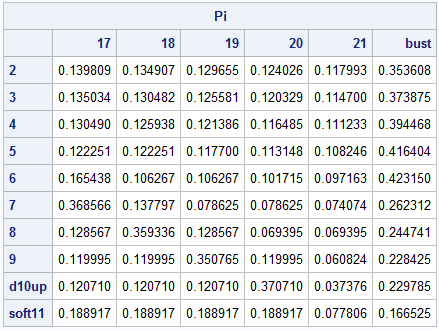
If you stare at these numbers long enough, you start to see some patterns, but the patterns become even more obvious if you instead use PROC SGPLOT to display this table as a heat map in which darker blue corresponds to higher probabilities:
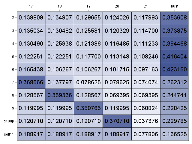
For example, when the dealer's up card is small, the most likely outcome is that the dealer will bust. Also, note that a dealer's up card of is most likely to yield a dealer total of
, and this matches the conventional wisdom to assume that the dealer's down card is a ten.
Armed with the dealer absorption probabilities, we can now move to the player's strategy, which is modeled as a Markov decision problem. Unlike the dealer, the player has several choices of actions, and the transition probabilities depend on the action. Let be the transition probability from state
to state
if player takes action
, and define value function
as the player's expected profit under optimal play, starting in state
. Then
satisfies Bellman's equation:
,
which we can again model by using linear programming (think of as the least upper bound):
This LP formulation applies to all Markov decision problems with finite state and action spaces, not just blackjack. The corresponding PROC OPTMODEL code is as follows, where the constraints are grouped by action and indicates if the player is (1) or is not (0) allowed to double down:
fix Pi; drop Recurrence Absorbing SumToOne; /* some lines omitted here */ var V {PLAYER_TOTALS, UP_CARDS, 0..1}; min Objective2 = sum {i in PLAYER_TOTALS, u in UP_CARDS, d in 0..1} V[i,u,d]; con Hit {i in NONPAIRS2, u in UP_CARDS, d in 0..1}: V[i,u,d] >= sum {c in CARDS} q[c] * V[pt_nonpairs[i,c],u,0]; con Stand {i in NONPAIRS2, u in UP_CARDS, d in 0..1}: V[i,u,d] >= sum {j in STANDING_TOTALS: points[j] < points[i]} Pi[u,j] - sum {j in STANDING_TOTALS: points[j] > points[i]} Pi[u,j]; con Double {i in NONPAIRS2, u in UP_CARDS}: V[i,u,1] >= 2 * sum {c in CARDS} q[c] * ( sum {j in STANDING_TOTALS: points[j] < points[pt_nonpairs[i,c]]} Pi[u,j] - sum {j in STANDING_TOTALS: points[j] > points[pt_nonpairs[i,c]] or pt_nonpairs[i,c] = 'bust'} Pi[u,j] ); con Split {i in PAIRS, u in UP_CARDS, d in 0..1}: V[i,u,d] >= if i ne 'pair1' then 2 * sum {c in CARDS} q[c] * V[pt_split[i,c],u,1] else 2 * sum {c in CARDS} q[c] * ( sum {j in STANDING_TOTALS: points[j] < points[pt_split[i,c]]} Pi[u,j] - sum {j in STANDING_TOTALS: points[j] > points[pt_split[i,c]]} Pi[u,j] ); con Nosplit {i in PAIRS, u in UP_CARDS, d in 0..1}: V[i,u,d] >= V[pt_nosplit[i],u,d]; con Bust {u in UP_CARDS, d in 0..1}: V['bust',u,d] = -1; |
A second SOLVE statement invokes the LP solver, which instantly returns the optimal solution. The following heat map shows the resulting optimal values of , where dark red is good for the player and dark blue is bad for the player. Each row corresponds to the player's hand
, and each column corresponds to the dealer's up card
.
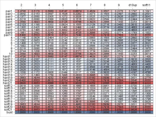
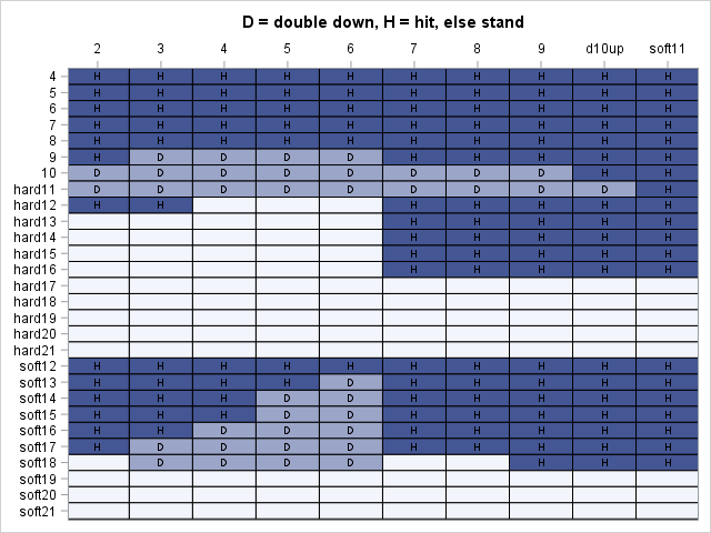
Again, several patterns are evident, but this imposing chart of expected profits defies memorization and is not practical for a player to use at the blackjack table. Instead, what the player really needs to know is the optimal action to take in each state, and this information is captured by the dual variables, whose values are accessible through the .DUAL constraint suffix. Explicitly, a positive dual value indicates that you should take the corresponding action. The following PROC OPTMODEL code prints the optimal strategy:
num epsilon = 1e-4; print '(Y = split, else do not split)'; print {i in PAIRS, u in UP_CARDS} ( if Split[i,u,1].dual > epsilon then 'Y' else ''); print '(D = double down, H = hit, else stand)'; print {i in NONPAIRS2, u in UP_CARDS} ( if Double[i,u].dual > epsilon then 'D' else if Hit[i,u,1].dual > epsilon then 'H' else ''); print '(H = hit, else stand)'; print {i in NONPAIRS2, u in UP_CARDS} ( if Hit[i,u,0].dual > epsilon then 'H' else ''); |
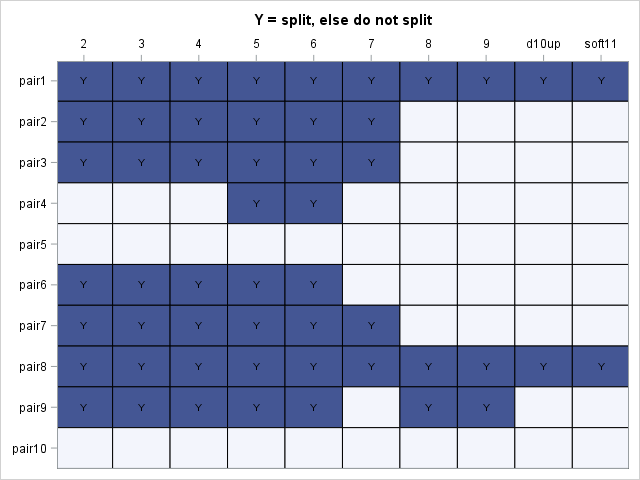
The optimal strategy for pairs is:
The optimal strategy if you can double down is:
The optimal strategy if you cannot double down is:
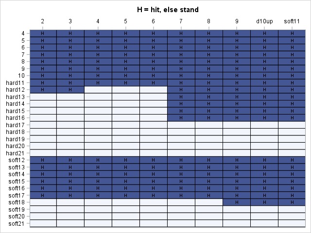
With enough practice, these tables are easy to memorize. In fact, casino gift shops sell wallet-sized versions of them, presumably to boost the confidence of would-be gamblers who might otherwise be intimidated by the pressure of making the correct decision only by gut feeling.
For more discussion and the full SAS code, see the SAS Global Forum 2011 paper Linear Optimization in SAS/OR® Software: Migrating to the OPTMODEL Procedure, which includes a calculation of the player's overall expected profit per hand. Spoiler alert: if you don't count cards, the expected profit is negative, but only slightly.
2 Comments
I play allot of blackjack. I know just about every commonly used card counting method. The one I like the best has a lower betting efficiency and a higher playing efficiency than the hi-low but counts considerably more card than the high-low. It's the ITA research method. 2-7+1 8 neutral 0 9-A-1. The problem I'm having with it although I've made many thousands of dollars with it, is that I'm unable to find a printed playing strategy. I've got everything from Wong and even an original copy of Lawrence Revere's playing blackjack as a business. Wong's halves count is beyond all doubt the most accurate in just about every way. However, counting halves and counting multiple different values is beyond my capabilities. Can you provide the actual playing strategy for the ITA research method?
The infinite-deck approximation used here ignores cards already dealt and hence yields a strategy that is not influenced by card counting. The counting method you mentioned is also known as Silver Fox, so you might find more information under that name.